YENEPOYA INSTITUTE OF TECHNOLOGY
NBA-Accredited : B.E (CSE & ME)
(Approved by AICTE, New Delhi, Affiliated to Visvesvaraya Technological University, Belgavi)
Department Details
Department Of Mathematics
Department of Mathematics was established in the year 2008 in order to provide a strong Mathematical foundation through course which cater to the needs of Mathematical applications for the students pertaining to the Engineering skills as well as higher education and research. We have dedicated, experienced and energetic faculty to impart invaluable information that may be used in both academic as well as professional life. At present, the department has one Associate Professor and five Assistant Professors. Our faculties are leaders in the fields of teaching and research activities. The department has more than 12 research publications in reputed national/international journals. The Department adopts various innovative techniques to improve the comprehension and problem solving skills of students.

Dr. M. Ajith Rao
Designation : Associate Professor
Qualification : B.Sc. M.Sc., M.Phil., Ph.D.
View Profile
.jpg)
Ms. Sashma C. H.
Designation : Assistant. Professor
Qualification : B.Sc., B.Ed. M.Sc., M.Ed.
View Profile

.jpg)


Vision
To strive to be recognized for academic excellence in the field of Mathematics through in-depth teaching and research, and to play a pivotal role in strengthening the ability of aspirants to solve engineering problems through mathematical problem solving techniques.
Mission
Making Engineers to develop mathematical thinking and applying it to solve complex engineering problems, designing mathematical modeling for systems involving global level technology.
Department Activities for Academic year 2022-2023:-
|
Event Name |
Duration |
Resource Person |
Organization |
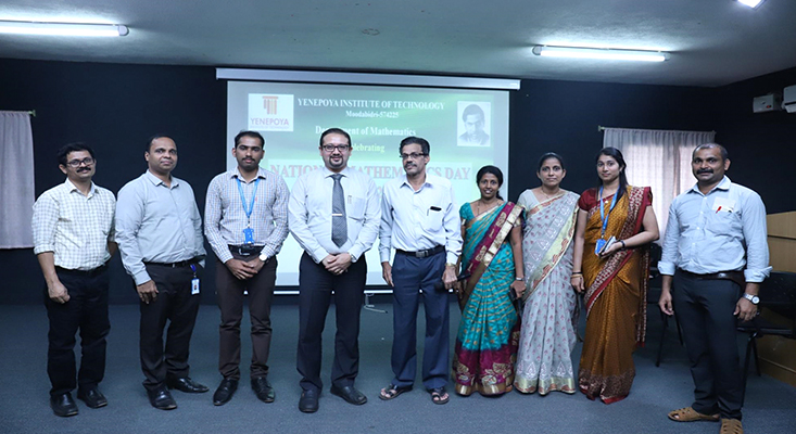
| INTERNATIONAL MATHEMATICS DAY | 11thMarch 2023, to 14thMarch 2023 | Dr. Ramanandha H S Dean – Student welfare, SJEC | YIT, Moodbidre |
Department Activities for Academic year 2020-2021:-
|
Event Name |
Duration |
Resource Person |
Organization |
|
A session on “ Ethics in Engineering Profession” |
3rd August,2021 to 5th August,2021 |
Ms. Likhitha B Shetty Assistant Professor, YIT- Moodbidri |
YIT, Moodbidri. |
|
A session on “ Ethical use of Chemicals” |
3rd August,2021 to 5th August,2021 |
Ms. Likhitha B Shetty Assistant Professor, YIT- Moodbidri |
YIT, Moodbidri. |
Department Activities for Academic year 2019-2020:-
|
Event Name |
Date |
Resource Person |
Organization |
|
A one day talk on “Life of Butterflies” |
31th October,2019 |
Speaker: Mr. Sammilan Shetty founder of ‘Sammilan shetty’s Butterfly park’ – Belvai
Coordinator: Ms. Shashirekha K Assistant Professor, Department of Engineering Chemsitry, YIT- Moodbidri |
YIT, Moodbidri. |
|
Webinar on “ Preparation of solution in the Engineering Laboratory and Common Challenges” |
14th June,2020 |
Speaker: Mr. Nagaraj P Associate Professor and Head, Department of Engineering Chemsitry, YIT- Moodbidri
Coordinator:Mr. Mohith Prasanna K Assistant Professor, Department of Engineering Chemsitry, YIT- Moodbidri |
YIT, Moodbidri. |
The department celebrated the National Mathematics Day - 2018 0n December 22 of 2018
Department Activities for Academic year 2015-2016:-
|
Event Name |
Date |
Resource Person |
Organization |
|
A one day talk on “Chemical ecology of Butterfly’’ |
18th September,2015 |
Speaker: Mr. Sammilan Shetty Founder of ‘Sammilan shetty’s Butterfly park’ – Belvai
Coordinator: Mr. Nagaraj P Assistant Professor and Head, Department of Engineering Chemsitry, Dr. M.V. Shetty Institute of Technology, (under Yenapoya management), Moodbidri |
Dr.M.V.Shetty Institute of Technology (under Yenapoya management), Moodbidri |
-
Mathematics-I for Electrical & Electronics Engineering Stream 2022
-
Mathematics-II for Electrical & Electronics Engineering Stream 2022
-
Mathematics-I for Mechanical Engineering stream 2022
-
Mathematics-II for Mechanical Engineering stream 2022
-
Mathematics-I for Computer Science and Engineering stream 2022
-
Mathematics-II for Computer Science and Engineering stream 2022
-
Syllabus 2021
-
Syllabus 2018
| Sr. No | Academic Year | Total Offers |
|---|